TechBlog 1

Basic intro and experiment of CV

In this blog, a simple CV process will be applied for object detection. From a basic image gradient vector, followed by image segmentation, and finally an example of object detection using VGG.

Image Gradient Vector

• Gradient: The direction of gradient is the greatest change rate of the function, which is used to find the extremum.

• Image Gradient Vector: Take the image as a function, gradient can be used to measure the pixel‘s change rate. Image gradient can be regarded as a two-dimensional discrete function, and image gradient is actually the derivative of this two-dimensional discrete function .

  $$\nabla f(x,y) = [G_x, G_y]^T = [{\partial f\over \partial x}, {\partial f\over \partial y}]^T$$

  Take the Sobel operator for an example, which mainly used for edge detection, is a discrete difference operator used to calculate the grayscale approximation of the image gradient function.

$$G_x = \left[ \begin{array}{ccc} -1 & 0 & 1 \\ -2 & 0 & 2 \\ -1 & 0 & 1 \end{array} \right] * A$$ $$G_x = \left[ \begin{array}{ccc} -1 & -2 & -1 \\ 0 & 0 & 0 \\ 1 & 2 & 1 \end{array} \right] * A$$

Calculation for an image .

• Image Process Example: here using an example to see the difference between applying and to process image pixel.
  The example image is:
  Code for this:

  import numpy as np
  import scipy
  import scipy.signal as sigs
  import matplotlib.pyplot as plt
  
  
  img = scipy.misc.imread("mygo1.jpg", mode="L")
  
  # Define the Sobel operator kernels.
  kernel_x = np.array([ [-1, 0, 1],[-2, 0, 2],[-1, 0, 1] ])
  kernel_y = np.array([ [1, 2, 1], [0, 0, 0], [-1, -2, -1] ])
  
  G_x = sig.convolve2d(img, kernel_x, mode='same')
  G_y = sig.convolve2d(img, kernel_y, mode='same')
  
  # Plot 
  fig = plt.figure()
  ax1 = fig.add_subplot(121)
  ax2 = fig.add_subplot(122)
  
  # the transformation (G_x + 255) / 2.
  ax1.imshow((G_x + 255) / 2, cmap='gray'); ax1.set_xlabel("Gx")
  ax2.imshow((G_y + 255) / 2, cmap='gray'); ax2.set_xlabel("Gy")
  plt.show()

  The result shows the comparation of using and .
  
  

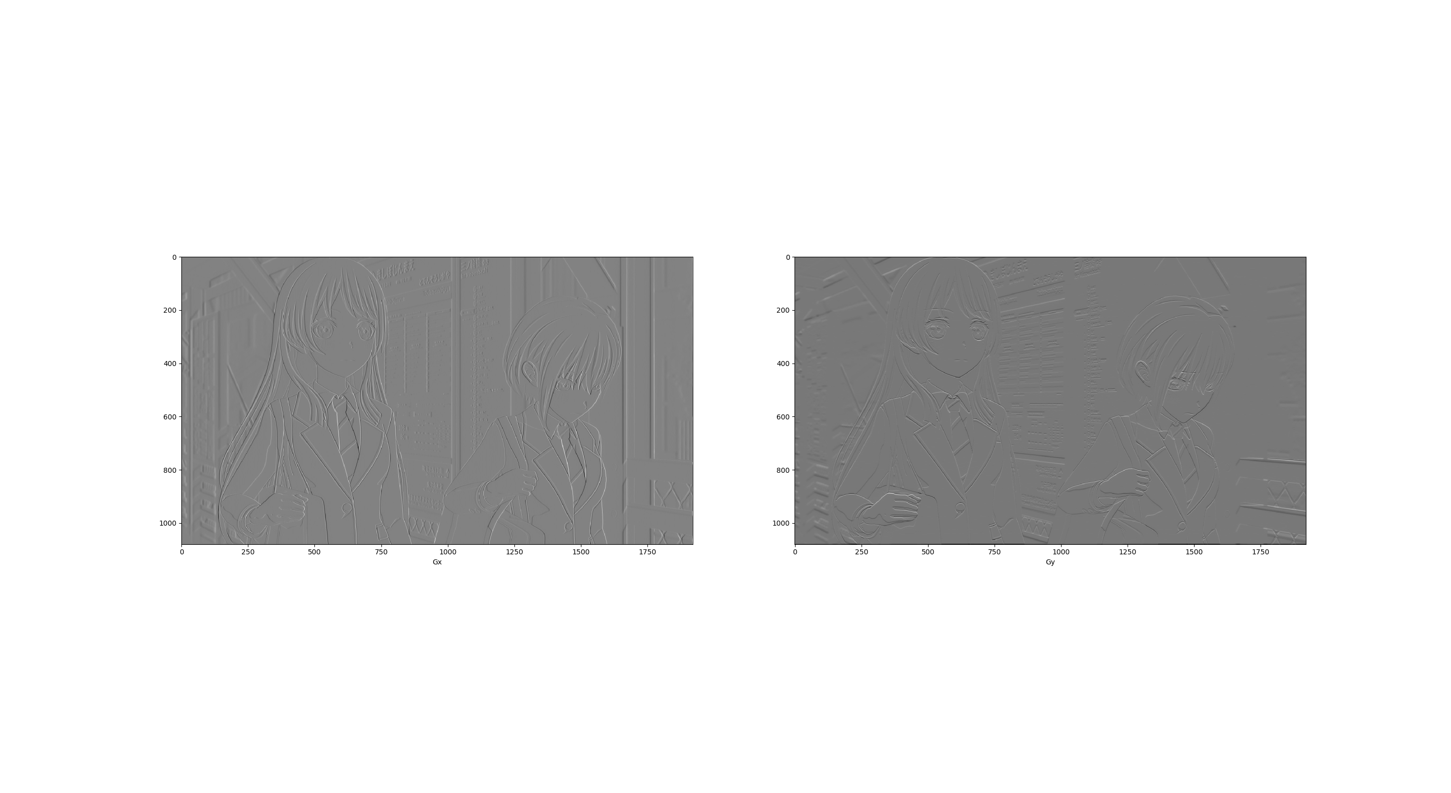
Image Segmentation

Felzenszwalb’s Algorithm was proposed for segmenting an image into similar regions. Each pixel is a vertex and then gradually merged to create a region, and the connection between each pixel is a minimum spanning trss (MST).

• How to Balance Difference bwtween two Pixels
  Difinations:

  • Internal Difference: , which represents the edge with the greatest dissimilarity in MST.
  • Difference between two components:
    , which represents the dissimilarity of the edge that connects all the edges of the two regions, the dissimilarity of the edge with the least dissimilarity. The dissimilarity of the two regions where they are most similar.

  The standard for merging two regions is:

  $$Diff(C_i, C_j) \lt Min(Int(C_i), Int(C_j))$$

  Only when and are able to stand the , they will be segmented into different regions. Otherwise, they are regarded as in the same region.
  

  • Procedures of the Algorithm
    Given , and .
    1. edges are sorted by dissimilarity (non-desconding), labeled as ,
    2. choose ,
    3. determines the currently selected edges for merging if meets:
       1)
       2) the degree of dissimilarity is not greater than the degree of dissimilarity within the two , then step 4. Otherwise, straight to step 5.
    4. update thresholds and class designators:
       class designators: -> ,
    5. if , select the next edge to go to step 3.

• Example Code
  Applying skimage segmentation to segment the example image. Set k = 100 and 500 to see how it controlls merge-region size for showing.
  
  The example image used for segmentation is:
  

  import numpy as np
  import scipy
  import scipy.signal as sig
  import skimage.segmentation
  from matplotlib import pyplot as plt
  
  img2 = scipy.misc.imread("iceland.jpg", mode="L")
  segment_mask1 = skimage.segmentation.felzenszwalb(img2, scale=100)
  segment_mask2 = skimage.segmentation.felzenszwalb(img2, scale=1000)
  
  fig = plt.figure(figsize=(12, 5))
  ax1 = fig.add_subplot(121)
  ax2 = fig.add_subplot(122)
  ax1.imshow(segment_mask1); ax1.set_xlabel("k=100")
  ax2.imshow(segment_mask2); ax2.set_xlabel("k=500")
  fig.suptitle("Felsenszwalb's efficient graph based image segmentation")
  plt.tight_layout()
  plt.show()

  Segment results (k = 100 & k = 500):
  

  Image Classification

• CNN for Image Classification
  Convolution operation: As we learned from the course, in short, convolution applies element-wise multiplication for the vector/ matrix and then
  summation.

• VGG (Visual Geometry Group)
  
  Using 3*3 convoluton layer and 2*2 pooling layer. VGG has two structures, namely VGG16 and VGG19, and there is no essential difference between the two, but the network depth is different.
  
  Why small size works better: each convolutional layer passes through an activation function. The activation function is a nonlinear transformation. The ability to be non-linear is stronger.
  

• Example Code
  
  Here I use VGG16 to implement a simple classficatoin for animals. The npy file and a class file for choosing results were downloaded from here.
  
  VGG16 contains 16 hidden layers (13 convolutional layers and 3 fully connected layers).
  
  The code for test is from here. I downloaded 3 images from google for test. Minor changed code for classifiication:

Click ME to Show Code

import numpy as np
import tensorflow.compat.v1 as tf
tf.disable_v2_behavior()
from scipy.misc import imread, imresize, toimage
import matplotlib.pyplot as plt
import skimage
import skimage.io
import skimage.transform
from imageClass import class_names

VGG_MEAN = [103.939, 116.779, 123.68]


class VGG16(object):
    """
    The VGG16 model for image classification
    """

    def __init__(self, vgg16_npy_path=None, trainable=True):
        """
        :param vgg16_npy_path: string, vgg16_npz path
        :param trainable: bool, construct a trainable model if True
        """
        # The pretained data
        if vgg16_npy_path is None:
            self._data_dict = None
        else:
            self._data_dict = np.load(vgg16_npy_path, encoding="latin1", allow_pickle= True).item()
        self.trainable = trainable
        # Keep all trainable parameters
        self._var_dict = {}
        self.__bulid__()

    def __bulid__(self):
        """
        The inner method to build VGG16 model
        """
        # input and output
        self._x = tf.placeholder(tf.float32, shape=[None, 224, 224, 3])
        self._y = tf.placeholder(tf.int64, shape=[None, ])
        # Data preprocessiing
        mean = tf.constant([103.939, 116.779, 123.68], dtype=tf.float32, shape=[1, 1, 1, 3])
        x = self._x - mean
        self._train_mode = tf.placeholder(tf.bool)  # use training model is True, otherwise test model
        # construct model
        conv1_1 = self._conv_layer(x, 3, 64, "conv1_1")
        conv1_2 = self._conv_layer(conv1_1, 64, 64, "conv1_2")
        pool1 = self._max_pool(conv1_2, "pool1")

        conv2_1 = self._conv_layer(pool1, 64, 128, "conv2_1")
        conv2_2 = self._conv_layer(conv2_1, 128, 128, "conv2_2")
        pool2 = self._max_pool(conv2_2, "pool2")

        conv3_1 = self._conv_layer(pool2, 128, 256, "conv3_1")
        conv3_2 = self._conv_layer(conv3_1, 256, 256, "conv3_2")
        conv3_3 = self._conv_layer(conv3_2, 256, 256, "conv3_3")
        pool3 = self._max_pool(conv3_3, "pool3")

        conv4_1 = self._conv_layer(pool3, 256, 512, "conv4_1")
        conv4_2 = self._conv_layer(conv4_1, 512, 512, "conv4_2")
        conv4_3 = self._conv_layer(conv4_2, 512, 512, "conv4_3")
        pool4 = self._max_pool(conv4_3, "pool4")

        conv5_1 = self._conv_layer(pool4, 512, 512, "conv5_1")
        conv5_2 = self._conv_layer(conv5_1, 512, 512, "conv5_2")
        conv5_3 = self._conv_layer(conv5_2, 512, 512, "conv5_3")
        pool5 = self._max_pool(conv5_3, "pool5")

        # n_in = ((224 / (2**5)) ** 2) * 512
        fc6 = self._fc_layer(pool5, 25088, 4096, "fc6", act=tf.nn.relu, reshaped=False)
        # Use train_mode to control
        fc6 = tf.cond(self._train_mode, lambda: tf.nn.dropout(fc6, 0.5), lambda: fc6)
        fc7 = self._fc_layer(fc6, 4096, 4096, "fc7", act=tf.nn.relu)
        fc7 = tf.cond(self._train_mode, lambda: tf.nn.dropout(fc7, 0.5), lambda: fc7)
        fc8 = self._fc_layer(fc7, 4096, 1000, "fc8", act=tf.identity)

        self._prob = tf.nn.softmax(fc8, name="prob")

        if self.trainable:
            self._cost = tf.reduce_mean(tf.nn.sparse_softmax_cross_entropy_with_logits(fc8, self._y))
            correct_pred = tf.equal(self._y, tf.argmax(self._prob, 1))
            self._accuracy = tf.reduce_mean(tf.cast(correct_pred, tf.float32))
        else:
            self._cost = None
            self._accuracy = None

    def _conv_layer(self, inpt, in_channels, out_channels, name):
        """
        Create conv layer
        """
        with tf.variable_scope(name):
            filters, biases = self._get_conv_var(3, in_channels, out_channels, name)
            conv_output = tf.nn.conv2d(inpt, filters, strides=[1, 1, 1, 1], padding="SAME")
            conv_output = tf.nn.bias_add(conv_output, biases)
            conv_output = tf.nn.relu(conv_output)
        return conv_output

    def _fc_layer(self, inpt, n_in, n_out, name, act=tf.nn.relu, reshaped=True):
        """Create fully connected layer"""
        if not reshaped:
            inpt = tf.reshape(inpt, shape=[-1, n_in])
        with tf.variable_scope(name):
            weights, biases = self._get_fc_var(n_in, n_out, name)
            output = tf.matmul(inpt, weights) + biases
        return act(output)

    def _avg_pool(self, inpt, name):
        return tf.nn.avg_pool(inpt, ksize=[1, 2, 2, 1], strides=[1, 2, 2, 1], padding="SAME",
                              name=name)

    def _max_pool(self, inpt, name):
        return tf.nn.max_pool(inpt, ksize=[1, 2, 2, 1], strides=[1, 2, 2, 1], padding="SAME",
                              name=name)

    def _get_fc_var(self, n_in, n_out, name):
        """Get the weights and biases of fully connected layer"""
        if self.trainable:
            init_weights = tf.truncated_normal([n_in, n_out], 0.0, 0.001)
            init_biases = tf.truncated_normal([n_out, ], 0.0, 0.001)
        else:
            init_weights = None
            init_biases = None
        weights = self._get_var(init_weights, name, 0, name + "_weights")
        biases = self._get_var(init_biases, name, 1, name + "_biases")
        return weights, biases

    def _get_conv_var(self, filter_size, in_channels, out_channels, name):
        """
        Get the filter and bias of conv layer
        """
        if self.trainable:
            initial_value_filter = tf.truncated_normal([filter_size, filter_size, in_channels, out_channels], 0.0,
                                                       0.001)
            initial_value_bias = tf.truncated_normal([out_channels, ], 0.0, 0.001)
        else:
            initial_value_filter = None
            initial_value_bias = None
        filters = self._get_var(initial_value_filter, name, 0, name + "_filters")
        biases = self._get_var(initial_value_bias, name, 1, name + "_biases")
        return filters, biases

    def _get_var(self, initial_value, name, idx, var_name):
        """
        Use this method to construct variable parameters
        """
        if self._data_dict is not None:
            value = self._data_dict[name][idx]
        else:
            value = initial_value

        if self.trainable:
            var = tf.Variable(value, dtype=tf.float32, name=var_name)
        else:
            var = tf.constant(value, dtype=tf.float32, name="var_name")
        # Save
        self._var_dict[(name, idx)] = var
        return var

    def get_train_op(self, lr=0.01):
        if not self.trainable:
            return
        return tf.train.GradientDescentOptimizer(lr).minimize(self.cost,
                                                              var_list=list(self._var_dict.values()))

    @property
    def input(self):
        return self._x

    @property
    def target(self):
        return self._y

    @property
    def train_mode(self):
        return self._train_mode

    @property
    def accuracy(self):
        return self._accuracy

    @property
    def cost(self):
        return self._cost

    @property
    def prob(self):
        return self._prob


# returns image of shape [224, 224, 3]
# [height, width, depth]
def load_image(path):
    # load image
    img = skimage.io.imread(path)
    img = img / 255.0
    # assert (0 <= img).all() and (img <= 1.0).all()
    # print "Original Image Shape: ", img.shape
    # we crop image from center
    short_edge = min(img.shape[:2])
    yy = int((img.shape[0] - short_edge) / 2)
    xx = int((img.shape[1] - short_edge) / 2)
    crop_img = img[yy: yy + short_edge, xx: xx + short_edge]
    # resize to 224, 224
    resized_img = skimage.transform.resize(crop_img, (224, 224))
    return resized_img


def test_not_trainable_vgg16():
    path = "D:/PyCharm Community Edition 2024.1.3/TechBlog"
    img1 = load_image(path + "/puppy.jpg") * 255.0
    batch1 = img1.reshape((1, 224, 224, 3))

    tf.compat.v1.disable_eager_execution()
    with tf.Graph().as_default(), tf.compat.v1.Session() as sess:
        vgg = VGG16(path + "/vgg16.npy", trainable=False)
        probs = sess.run(vgg.prob, feed_dict={vgg.input: batch1, vgg.train_mode: False})
        for i, prob in enumerate([probs[0]]):
            preds = (np.argsort(prob)[::-1])[0:5]
            print("The" + str(i + 1) + " image:")
            for p in preds:
                print("\t", p, class_names[p], prob[p])


if __name__ == "__main__":
    path = "D:/PyCharm Community Edition 2024.1.3/TechBlog"
    img1 = load_image(path + "/puppy.jpg") * 255.0
    batch1 = img1.reshape((1, 224, 224, 3))
    x = np.concatenate((batch1), 0)
    y = np.array([292, 611], dtype=np.int64)
    with tf.Graph().as_default():
        with tf.Session() as sess:
            vgg = VGG16(path + "/vgg16.npy", trainable=True)
            sess.run(tf.global_variables_initializer())

            train_op = vgg.get_train_op(lr=0.0001)
            _, cost = sess.run([train_op, vgg.cost], feed_dict={vgg.input: x,
                                                                vgg.target: y, vgg.train_mode: True})
            accuracy = sess.run(vgg.accuracy, feed_dict={vgg.input: x,
                                                         vgg.target: y, vgg.train_mode: False})
            print(cost, accuracy)
 

Example images for VGG16:

1. Puppy
   
   
   
   The results generated by VGG16 for the puppy was a “Japanese spaniel“.

2. Cat
   
   
   
   The results generated by VGG16 for this cat was a “Egyptian cat“.

3. Saber
   
   
   
   Sadly, it only implements object detection known in the class file to the image instead of recognition of Saber. To make it successful, dataset for her needs to be collected for training.
   

In the next Blog, I intend to apply YOLO for image classification, from training dataset to realize the image recognition. Hopefully, Saber will be recognized :).

Reference

[1] Gradient Vector

[2] Pedro F. Felzenszwalb, and Daniel P. Huttenlocher. “Efficient graph-based image segmentation.” Intl. journal of computer vision 59.2 (2004): 167-181.article

[3] 图像分割—基于图的图像分割 blog address

[4] Simonyan, K. (2014). Very deep convolutional networks for large-scale image recognition. arXiv preprint arXiv:1409.1556.

[5] VGG in TensorFlow